Deep learning model performance depends on the quality and size of the training dataset. But collecting high-quality, diverse, and accurately labeled data is costly and slow.
Also, the real world is full of chaos and variability. Data gathered in a controlled space rarely captures all the different lighting, obstacles, and conditions a model will face when put into actual use.
Data augmentation solves this by artificially expanding and bringing diversity to your limited training data. It’s a fast and scalable way to improve model generalization for computer vision tasks like image classification, object detection, and image segmentation.
In this guide, we will cover:
- What is data augmentation, and why is it important?
- Image data augmentation techniques (basic + advanced)
- Offline vs. online data augmentation
- Data augmentation best practices
- Real-life applications and use cases
- Tools and Libraries for Data Augmentation in Computer Vision
- Challenges of data augmentation
- How Unitlab can help with data augmentation and management
If you want to improve the quality of your domain-specific vision datasets through data augmentation, use Unitlab. It lets you generate augmented versions of your images without leaving the platform or writing custom scripts.
Interested in trying Unitlab? Try it out for free!
Figure 1: Annotate, augment, and manage your data in Unitlab.
What Is Data Augmentation?
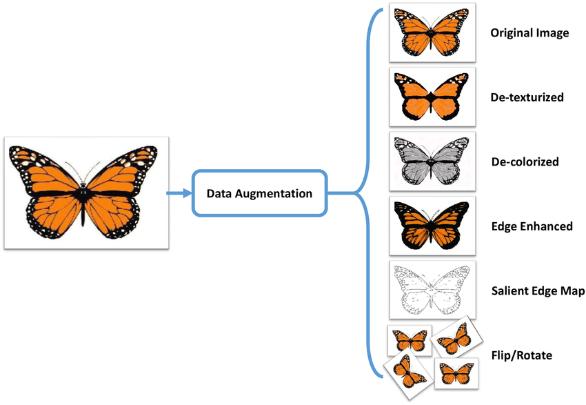
Data augmentation is a technique to transform existing input images (or other data) to create new, altered samples.
In effect, augmentation increases the size and diversity of the dataset without additional data collection.
For example, we can take an original photograph and produce rotated, flipped, or color-modified versions of it. And these variations are treated as new training examples.
Data augmentation solves data scarcity in many specialized computer vision fields, like medical imaging or industrial inspection, where collecting enough real data samples is difficult.
Why Is Data Augmentation Important for Deep Learning?
Data Augmentation comes into play whenever your dataset is limited or may not fully represent real-world variability.
Here’s why it matters:
- Preventing Overfitting: Augmented data introduces variability and randomness, so models cannot memorize training images. When the model sees many slightly different versions of the same sample data, it learns more general patterns instead of focusing on noise.
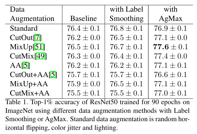
- Improving Generalization: Augmented data improves model generalization by exposing neural networks to the kinds of variations they will see in real-world data. In fact, this paper reports up to 1.5% improvement in top-1 accuracy on ImageNet (using ResNet-50) compared to the baseline when using augmented data plus AgMax regularization.
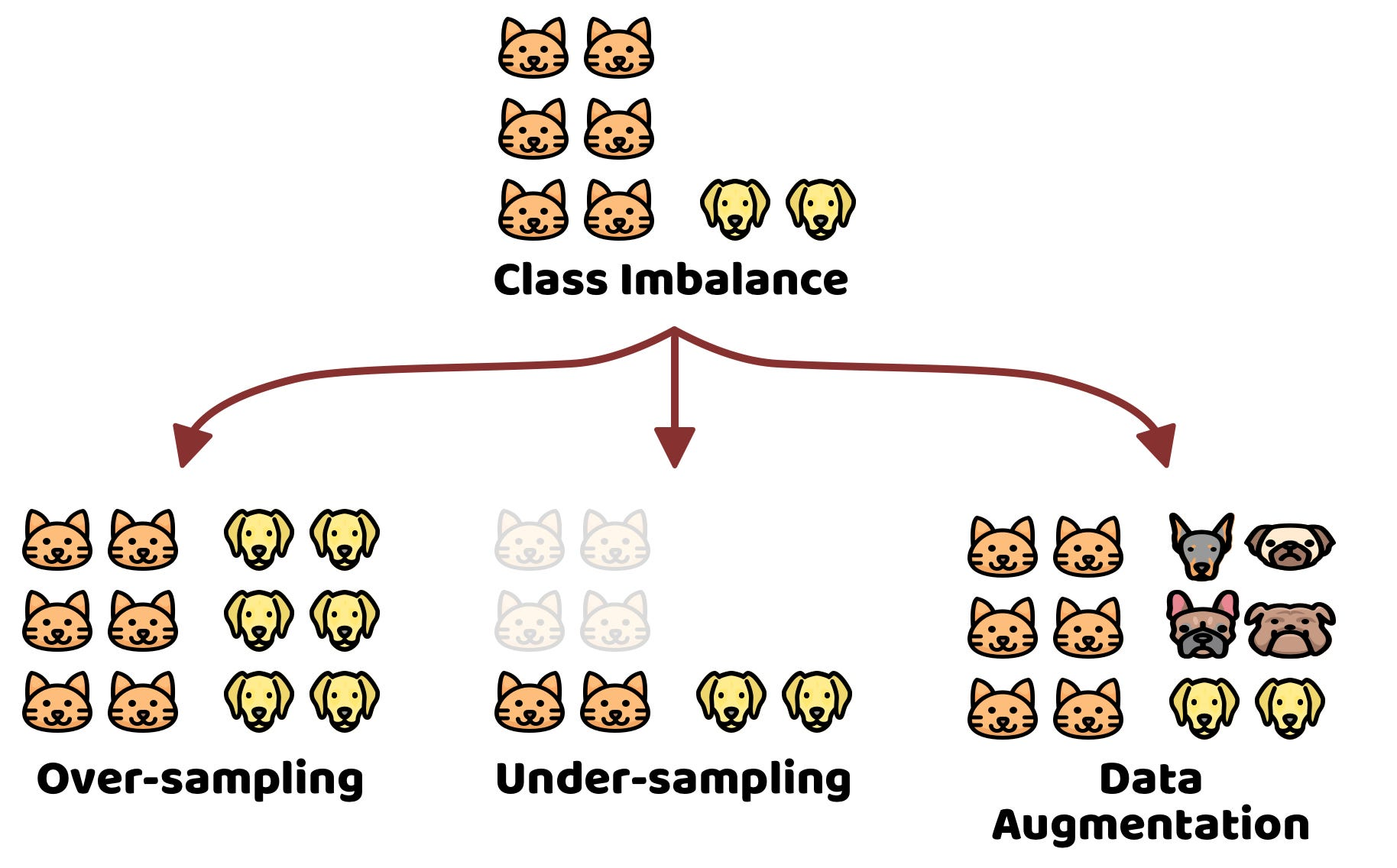
- Addressing Class Imbalance: When some classes are underrepresented, models may perform poorly on them. Augmentation oversamples minority classes by creating more examples (augment images of a rare object with more variations).
Common Image Data Augmentation Techniques in Computer Vision
While data augmentation techniques vary depending on the specific problem you are solving, many are simple image processing operations that are easy to implement. These techniques work across common computer vision tasks.
Geometric Transformations
Geometric transformations alter the spatial layout of an image while preserving its semantic meaning. Typical operations include:
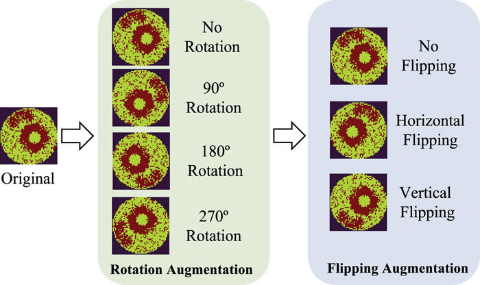
- Flipping: Random horizontal (and sometimes vertical) flips mirror the image without changing the label. For example, a horizontal flip creates a left-right mirrored copy. But when using vertical flipping, we need more care, since some domains, such as medical imaging, may treat upside-down content as unrealistic (domain-dependent).
- Rotation: Rotating images by small random angles theta ( ±45°) simulates different viewpoints and helps models handle cases where objects are not perfectly aligned.
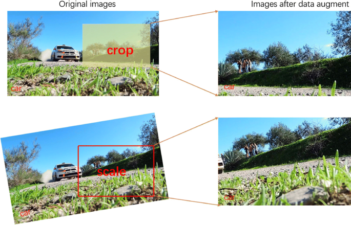
- Cropping and Zooming: Cropping extracts a random sub-region of the original image and resizes it to the input dimension. It also simulates partial occlusion. On the other hand, zooming in or out on the image simulates variability in object distance. A model trained with random zooming learns to detect the object, whether it occupies 10% of the frame (far away) or 90% of the frame (close up), to ensure scale invariance.
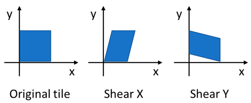
- Shearing: Shearing applies a non-affine transformation that shifts one part of an image along an axis to introduce perspective changes while holding the other fixed. It is handy in OCR to handle italicized or slanted handwriting.
Photometric (Color) Transformations:
Photometric transformations change pixel intensities and color properties while keeping the scene structure intact.
Common operations include:
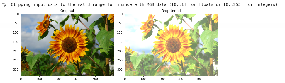
- Brightness and Contrast Adjustment: It involves brightness adjustment (randomly brightening or darkening an image) or altering contrast to mimic different lighting conditions. For instance, increasing brightness helps the model cope with sunny conditions, and darkening simulates shadows.
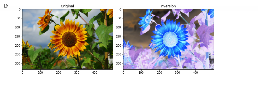
- Color Jitter and Saturation Changes: Random changes to hue, saturation, or color balance teach the model invariance to color shifts.
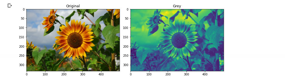
- Grayscale Conversion: Sometimes, converting to grayscale (or mixing grayscale and color) can help the model be less sensitive to color.
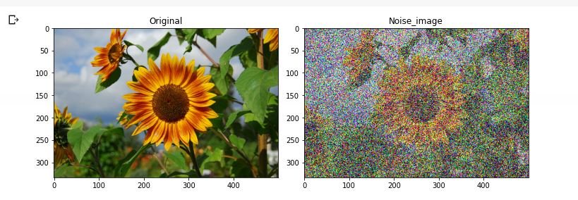
- Gaussian Noise Injection: Adding random Gaussian noise simulates sensor noise or low-light grain.
Each of these methods alters pixel values while preserving the object. They are widely used alongside geometric changes to further enrich the dataset.
Now, let's discuss the advanced image data augmentation methods.
Advanced Data Augmentation Techniques and Generative AI
Modern computer vision employs advanced image data augmentation methods beyond the basic transforms. These techniques mix data samples or use generative models to create new data and can considerably improve the model performance.
Mixing Images
Mixing techniques produces images that look unrealistic to human observers, yet they improve model robustness and performance. Some of the mixing techniques are:
- MixUp: MixUp creates a new training example by taking a weighted average of two random images and likewise mixing their labels. If we take an image of a cat (x₁) and a dog (x₂), create a new image and a mixed label using the same weight. Here is the formula to mix images:

The label is also mixed:

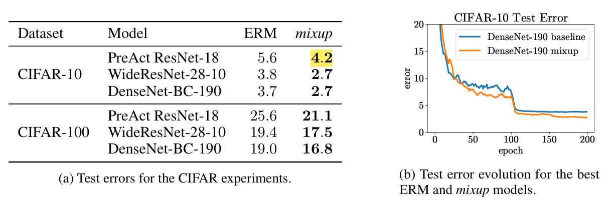
- According to the original paper, MixUp reduces test error from about 5.6% to 4.2% (an absolute improvement of about 1.3% points) on CIFAR‑10.
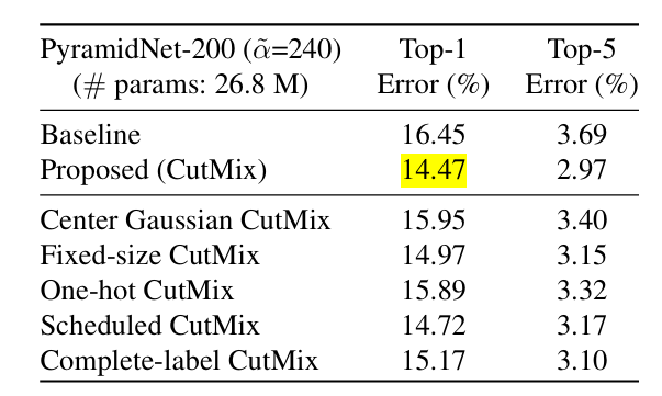
- CutMix: CutMix is similar but replaces a rectangular patch (cutout) from one image and pastes it onto another, and combines labels proportionally. The label is adjusted based on the proportion of pixels belonging to each class. CutMix combines the benefits of regional dropout (forcing the model to look at other parts of the image) with the efficiency of training on two classes in parallel.
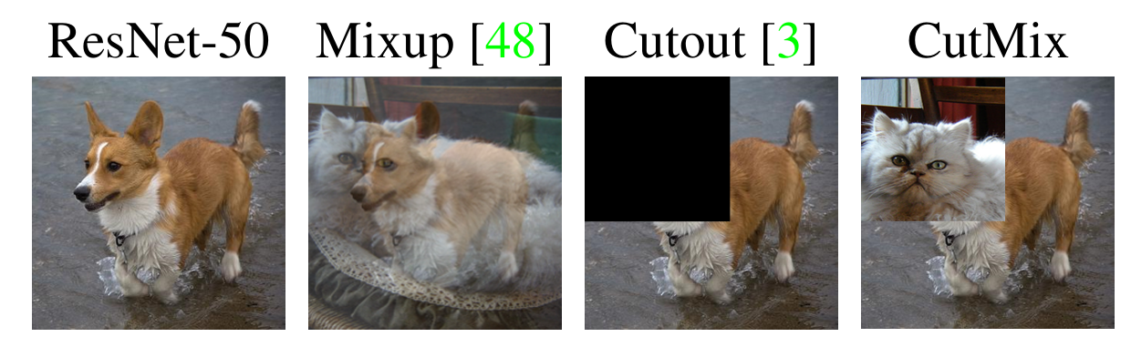
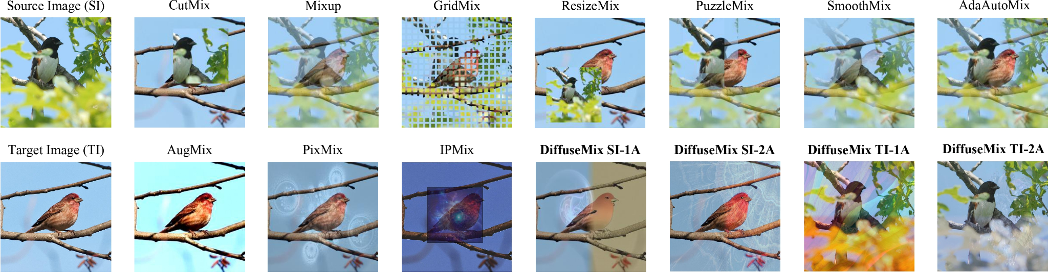
Figure 14: Comparison of different data augmentation techniques.
- In fact, adding CutMix to ResNet‑50 on the ImageNet classification task improves top‑1 accuracy by about 2.3% points over the baseline. And on CIFAR‑100, CutMix reduces top‑1 error from 16.45% to 14.47% (about a 2‑point absolute improvement).
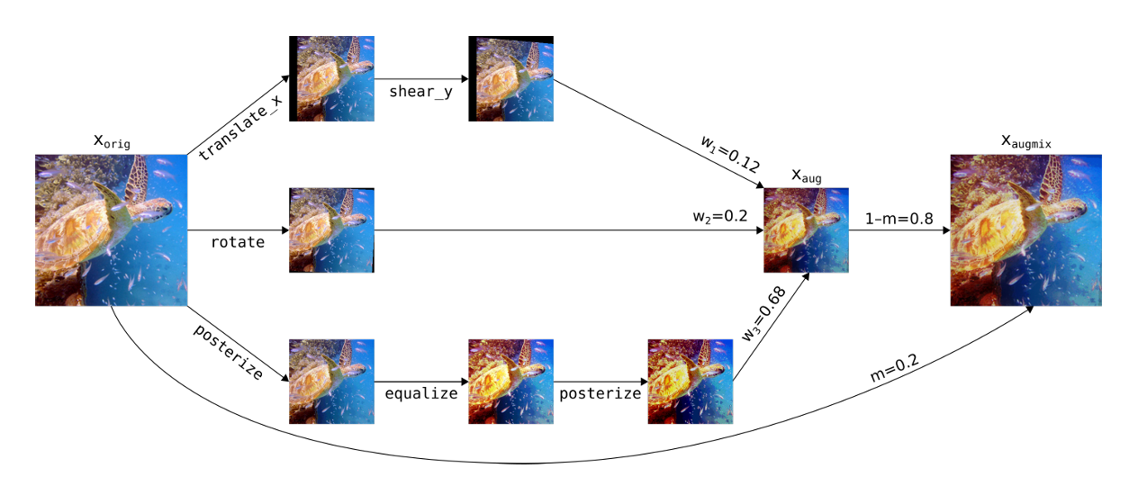
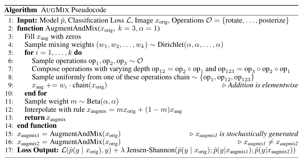
- AugMix: It improves models against corruptions (blur, noise, compression). It mixes different augmented versions of the same image. An image is split into several chains of augmentations (rotate then shear; contrast then blur). These chains are then mixed together with the original image using a weighted average.
- The AugMix algorithm is provided below in pseudocode.
- Mosaic Augmentation: Mosaic stitches four different images into a single 2x2 grid, then randomly crops it. Mosaic improves upon CutMix for object detection model as it effectively shows multiple contexts in one image by resizing and randomly cropping from the tiled result.
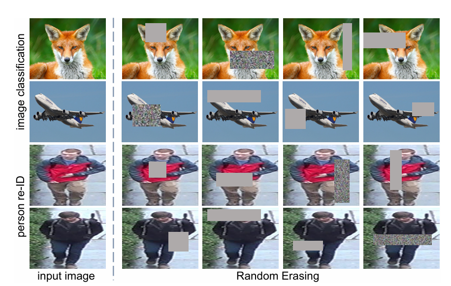
Random Erasing (Cutout) in the Image
Random Erasing (also known as Cutout) randomly selects a rectangle region in an image and erases its pixels (fills with noise or constant values).
This trains the model to recognize objects even when parts are missing or occluded, similar to real world scenarios where objects are blocked by other items or cut off by the frame.
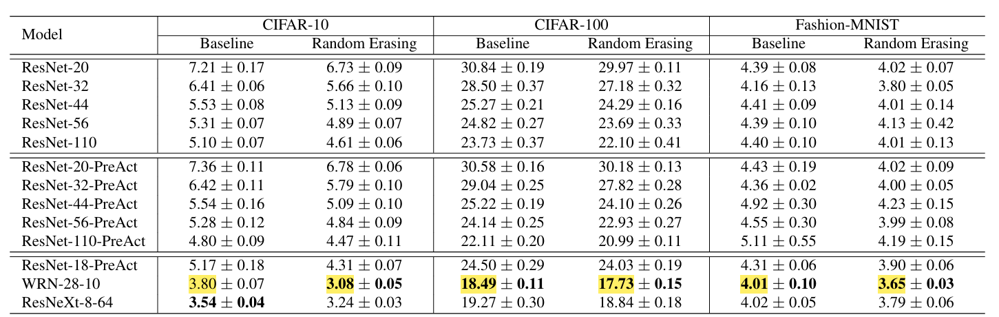
As per the paper, Random Erasing improves WideResNet‑28‑10 on CIFAR‑10 from about 3.80% test error to 3.08% and on CIFAR‑100 it reduces error from roughly 18.49% to 17.73%.
While on Fashion‑MNIST, it lowers top‑1 error from 4.01% to 3.65%, showing consistent but modest boosts in accuracy across different datasets.
Automated Augmentation Search
Methods like AutoAugment (introduced by Google Brain) and RandAugment use learning algorithms to find the best data augmentation policies.
For instance, AutoAugment uses reinforcement learning to search for augmentation combinations.
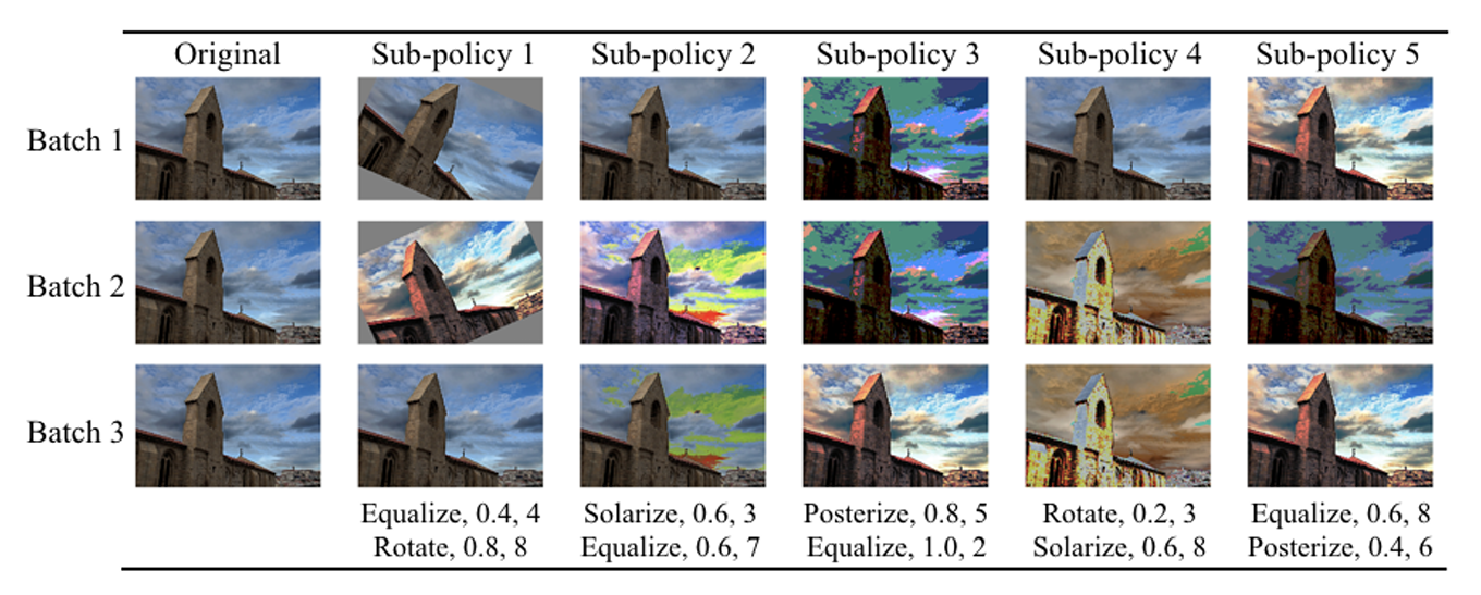
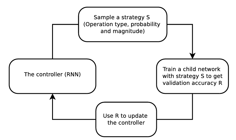
A controller neural network (RNN) proposes an augmentation policy (a set of operations like shear, rotate, along with their probabilities and magnitudes).
A child model is trained with this policy, and its validation accuracy serves as the reward signal for updating the controller.
Over time, the controller learns the optimal data augmentation strategy for the specific dataset. But implementing the AutoAugment is computationally expensive (requiring thousands of GPU hours to search).
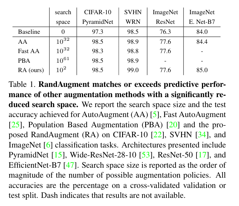
RandAugment simplified the approach. It defines a unified search space and simply selects a random subset of transformations with a single global magnitude parameter instead of learning a policy.
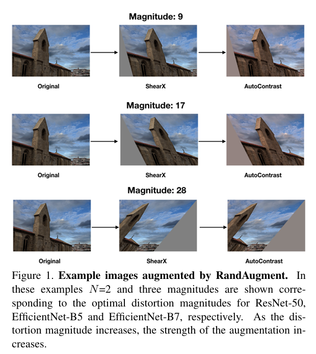
Surprisingly, this random strategy matches the performance of learned policies, as the paper showed RandAugment gave ~0.4% improvement over AutoAugment.
Also, it achieved 1.0% higher top-1 accuracy over baseline augmentation on ImageNet (with EfficientNet-B7).
Generative Models (GANs, Diffusion, Style Transfer)
Data augmentation techniques based on Generative adversarial networks (GANs) and diffusion models can synthesize entirely new training images. These approaches learn the sample data distribution and generate realistic samples to expand the synthetic data available for training.
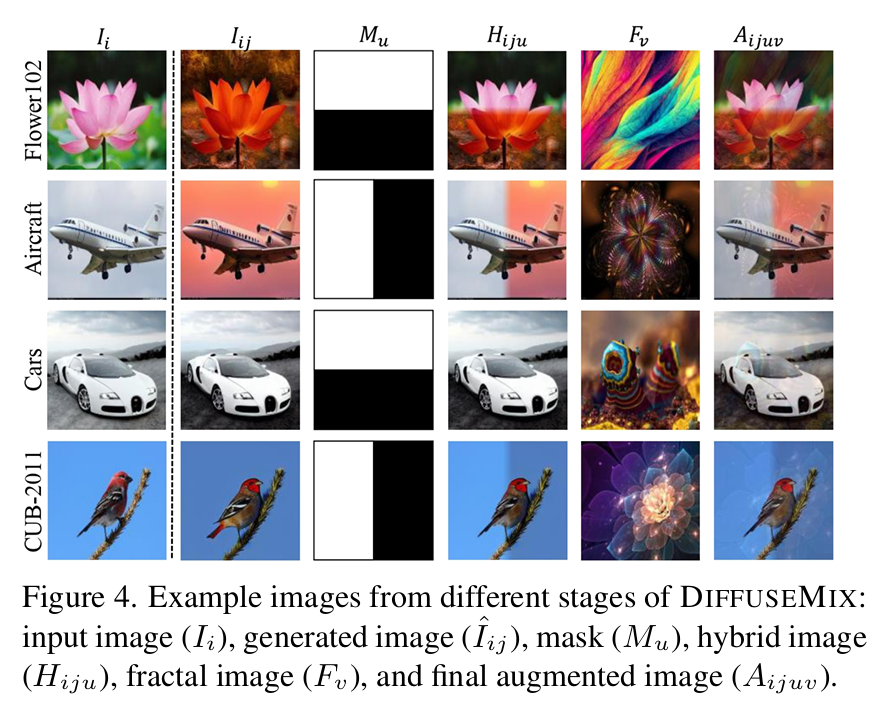
For example, DiffuseMix uses generative models to generate new images in a label-preserving way. Instead of mixing two images (which can introduce ambiguity), it expands each original image with a generated counterpart plus an optional structural overlay.
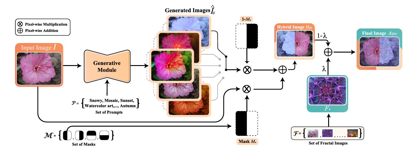
The paper mentioned that when evaluated on several classification datasets, DiffuseMix achieves superior performance compared to existing state-of-the-art methods.
Offline vs. Online Data Augmentation Implementation
Data augmentation can be implemented offline or online, depending on how and when the transformations are applied. Each approach has trade-offs in terms of disk usage, flexibility, and training speed.
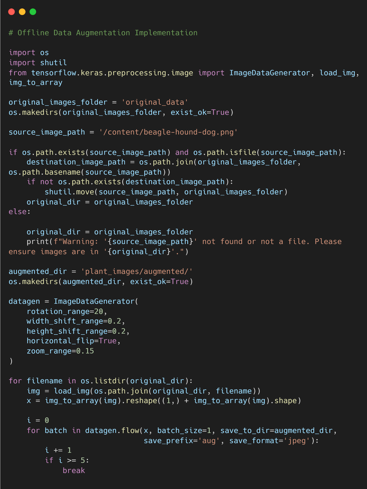
Offline augmentation means pre-generating augmented images and saving them to disk before the model training begins.
You apply transforms to each image in your dataset (possibly many times) and build a larger directory of images. Training then simply reads from this expanded set.
The advantage is that the augmented dataset is fixed, and all images are known in advance. The downside is a huge storage cost (generating 10× more images will use 10× the disk space).
It also lacks variability, as once images are generated, training always sees the same augmented samples.
Here is the code example to implement offline image data augmentation.
On the other hand, online (on-the-fly) augmentation applies random transformations to images in real time during training. Each time an image is loaded (each epoch or batch), a random transform is applied.
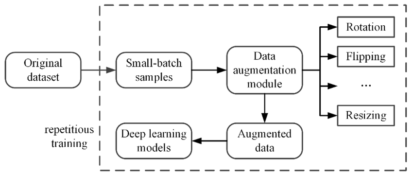
For example, a random flip or crop is applied on-the-fly with some probability. We program augmentation into the data loading pipeline. The model thus sees a different version of the image each epoch, effectively an infinite set of variations.
This requires no extra storage, but it does slightly slow down training (since transformations happen in memory per batch).
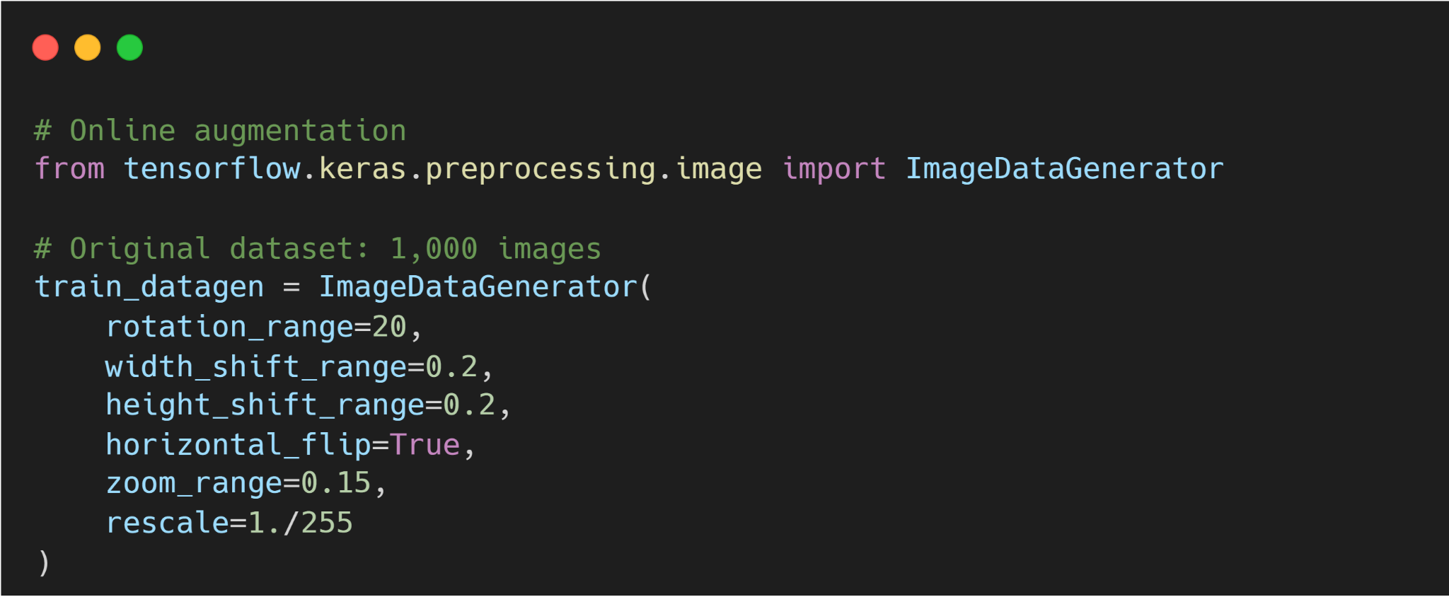
Here is a sample code for implementing online image augmentation.
Data Augmentation Best Practices
Here are key practices when applying data augmentation:
- Match Augmentations to the Task Type: Choose augmentation methods that make sense for your data and problem. Avoid transformations that change the image's semantics (flipping handwritten 6 into 9).
- Start Simple, Ramp Up Slowly: Start with mild augmentations and increase intensity gradually. Avoid excessive use to prevent artifacts and performance issues. Also, monitor your model’s accuracy, and if it drops after an augmentation, scale back.
- Maintain Data Integrity: Always verify that augmented images still match their original labels. Keep some original data un-augmented as a control to ensure that your model still performs well on real (unaugmented) images.
- Validate with a Test Set: Data augmentation can improve training accuracy, but only validation on real data tells you if it truly generalizes. Perform ablation studies by adding one type of augmentation at a time.
- Balance the Dataset: If class imbalance is an issue, consider applying augmentations more heavily to minority classes.
- Use Efficient Pipelines: Implement augmentation using efficient libraries and parallel data loading to avoid bottlenecks. If training slows down due to augmentation, consider simpler transforms or more optimized tools.
Real-World Image Data Augmentation Applications and Use Cases
Data augmentation is widely used in production systems across machine learning tasks. The right augmentation strategy depends on the domain and the type of input data.
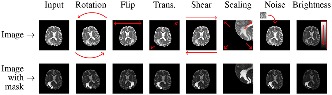
Medical Imaging
Labeled data is often scarce due to privacy constraints, the cost of expert annotation, and regulatory limits on data sharing in medical domains like medical image analysis.
Image data augmentation using rotation, scaling, flipping, and elastic deformations can generate varied yet realistic training images from a small existing dataset.
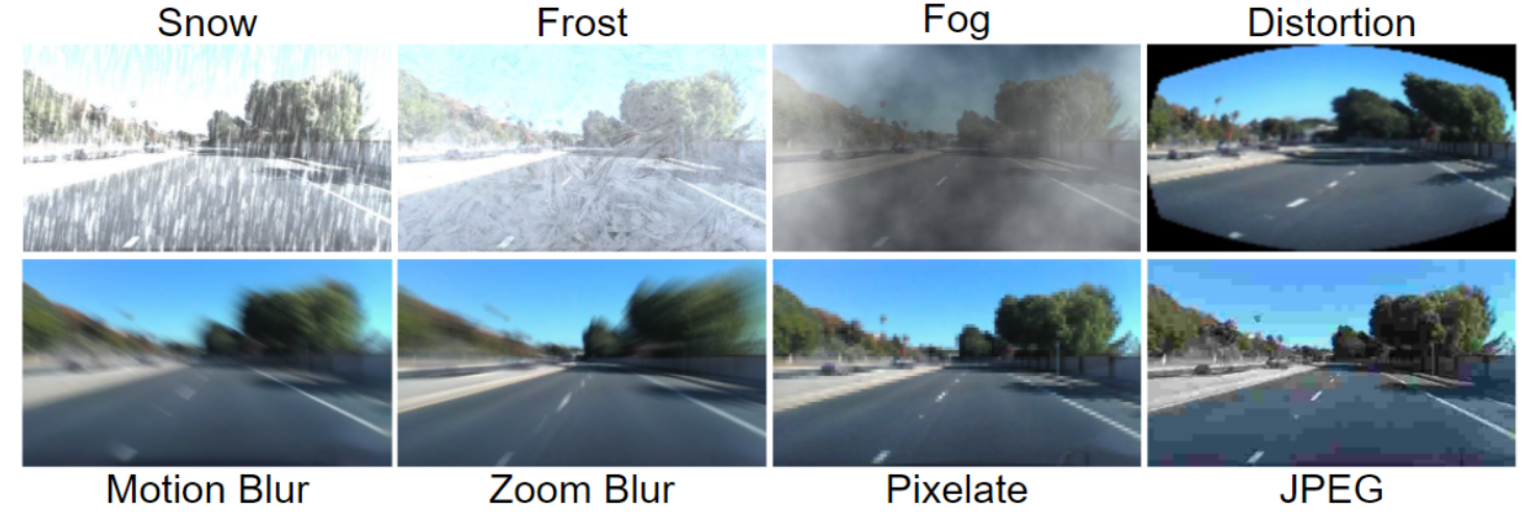
Autonomous Driving
Self-driving cars see the world under wildly varying conditions (day vs. night, sunny vs. rainy). Augmentation helps train vision systems for these scenarios.
For instance, brightness and contrast adjustments simulate different lighting (sun glare or shadows).
Synthetic overlays like fog, rain streaks, or snow can also be added to images to teach models to perceive through adverse weather.
In fact, data from driving simulators or GAN-generated weather conditions are often mixed into real driving datasets.
The goal is that the object detector and segmentation models learn to recognize road signs, pedestrians, and obstacles under any weather or lighting conditions.
Optical Character Recognition (OCR) and Document Scanning
OCR systems must handle many fonts, handwriting styles, and scanning artifacts. Common augmentations include adding noise, blur, and elastic distortions to text images. This mimics real-world factors like low-quality scans or camera blur.
Random pixel noise (salt-and-pepper or Gaussian) makes the model tolerant to grainy images. But, flipping text images is avoided in OCR since flipping letters vertically or horizontally would make them unreadable. Instead, slight rotations or warping are used to simulate tilted pages.
If you are working on any of these domains and you are struggling with limited data, and getting more data is expensive, then you can use Unitlab image augmentation toolkit.
It allows you to label the data and apply data augmentations interactively, such as rotation and zooming, to improve the model's detection performance from different angles.
Tools and Libraries for Data Augmentation in Computer Vision
Most deep learning frameworks make implementing data augmentation pipelines easier by providing many basic and advanced techniques. Some tools include:
- Torchvision (PyTorch): A standard library of image transforms for PyTorch. It includes many built-in augmentations (flips, crops, color jitter) that can be chained together. Torchvision transforms are easy to use with DataLoader to implement online augmentation.
- Unitlab Image Augmentation Toolkit: Unitlab includes a built-in image augmentation toolkit directly inside the annotation platform. You can generate augmented versions of your images that help increase dataset diversity, balance rare classes, and speed up experimentation while you annotate and manage data in one place.
- Albumentations: It offers over 100 transforms (both geometric and pixel-level adjustments) and is optimized for performance. Albumentations supports bounding boxes, masks, and multi-task augmentations, and the API is similar to torchvision and works with NumPy arrays or tensors.
- Imgaug: Imgaug lets you combine multiple augmentations, use them in random order, and even augment keypoints, bounding boxes, and heatmaps alongside the image. It supports operations on multiple CPU cores and provides a stochastic interface for fine-grained control.
- Keras ImageDataGenerator: With the ImageDataGenerator class, you can perform basic transforms (rotation, shifting, zoom, flips) and can be used with flow_from_directory to train models with augmented data. While less flexible than Albumentations or Imgaug, it is simple to use for common cases in Keras.
Challenges of Data Augmentation
While data augmentation can improve model performance, misuse or overuse can lead to unintended side effects. Here are some practical limitations:
- Increased Computational and Storage Complexity: Augmenting data on-the-fly increases the computational cost of training. On the other hand, offline augmentation multiplies storage needs. ML engineers face the trade-off between on-the-fly (slower but no storage cost) and precomputed (fast but storage-heavy).
- Bias Propagation: If the base dataset has errors or biases, augmenting it will propagate those issues. Moreover, poorly chosen transformations can break semantic meaning.
- Label Integrity Risk: Certain transformations, like flipping digits or rotating medical images, may invalidate the label.
- No New Information: The augmentation process uses existing data, meaning no fundamentally new patterns are introduced.
- Finding the Right Strategy: There is no one-size-fits-all augmentation. Effective methods depend on the data and task. Experimentation is required to find what helps versus what hurts.
How Unitlab AI Can Help with Data Augmentation and Management Needs
Unitlab helps teams turn augmentation into a controlled, end‑to‑end workflow instead of a disconnected scripting task.
Augmentation multiplies the amount of image data, but high‑quality labeling and dataset management remain the real bottlenecks.
So Unitlab combines AI‑assisted annotation with an in‑platform augmentation toolkit to govern the full cycle from clean seed labels to large augmented training sets.
Here is how the Unitlab data pipeline works:
- First, Unitlab ensures the quality of ground truth using the Segment Anything Model assistance. Tools like Magic Touch provide one-click, precise segmentation, and Batch Auto-Annotation propagates labels across similar images to build a strong base dataset up to 15x faster.
- Once this foundation is in place, Unitlab's integrated augmentation toolkit lets you to generate augmented image versions within the platform. Since augmentation lives next to labeling, you can keep track of which images are original, which are augmented, and how each set contributes to the final training dataset.
- Unitlab reduces the operational cost of scaling vision datasets through dataset management in the same UI. You can spend less time shuffling files and more on tuning machine learning models, and analyzing results, while retaining clear traceability from raw data to final training sets.
Conclusion
Data augmentation simulates new data points, avoids overfitting, and prepares your model for real-world variability.
Using a combination of simple augmentations (flips, crops, color jitter) and advanced methods will extract the maximum value from your original dataset.
Pair these techniques with best practices and the right tools, and you’ll dramatically enhance your training set.
Starting with a solid, well-labeled base using Unitlab’s annotation platform ensures that the augmented images remain reliable.